本文为清华大学”模式识别与机器学习”课程的复习笔记。
Evaluation Metric
k-NN
Nearest Neighbor
For a new instance $x’$, its class $\omega’$ can be predicted by:
k-Nearest Neighbor
For a new instance $x$, define $g_i(x)$ as: the number of $x$’s k-nearest instances belonging to the class $\omega_i$.
Then the new instance’s class $\omega’$ can be predicted as:
k-NN Improvements
Branch-Bound Algorithm
Use tree structure to reduce calculation.
Edit Nearest Neighbor
Delete nodes that may be misguiding from the training instance set.
Condensed Nearest Neighbor
Delete nodes that are far away from decision boundaries.
The Curse of Dimensionality
Problem
- Many irrelevant attributes
- In high-dimensional spaces, most points are equally far from each other.
Solution
- Dimensionality reduction techniques
- manifold learning
- Feature selection
- Use prior knowledge
Linear Regression (Multivariate ver.)
For a multivariate linear regression, the function becomes $ y_i = \mathbf{w}^{\rm T}\mathbf{x}_i $ , where $ \mathbf{x}_i = (1, x_i^1, \cdots, x_i^d)^{\rm T}\in \mathbb{R}^{d+1}, \mathbf{w} = (w_0, w_1, \cdots, w_d)^{\rm T} \in \mathbb{R}^{d+1}$, We adjust the values of $\mathbf{w}$ to find the equation that gives the best fitting line $f(x) = \mathbf{w}^{\rm T}\mathbf{x}$
We find the best $ \mathbf{w}^*$ using the Mean Squared Loss: $\ell(f(\mathbf x, y)) = \min\limits_{\mathbf w} \frac{1}{N} \sum_{i = 1}^N (f(\mathbf x_i) - y_i)^2 = \min \limits_{\mathbf w} \frac{1}{N}(\mathbf {Xw-y})^{\rm T}(\mathbf {Xw-y})$
So that $ \mathbf{w}^{\star} $ must satisfy $ \mathbf {X^{\rm T}} \mathbf {Xw^{\star}} = \mathbf X^{\rm T}\mathbf y$ , so we get $\mathbf{w^{\star}} = (\mathbf {X^{\rm T}X})^{-1}\mathbf X^{\rm T}\mathbf y$ or $\mathbf{w^{\star}} = (\mathbf {X^{\rm T}X} + \lambda \mathbf I)^{-1}\mathbf X^{\rm T}\mathbf y$ (Ridge Regression)
Linear Discriminant Analysis
project input vector $\mathbf x \in \mathbb{R}^{d+1}$ down to a 1-dimensional subspace with projection vector $\mathbf w$
The problem is how do we find the good projection vector? We have Fisher’s Criterion, that is to maximize a function that represents the difference between-class means, which is normalized by a measure of the within-class scatter.
We have between-class scatter $\tilde{S}_b = (\tilde{m}_1 - \tilde{m}_2)^2$, where $\tilde{m}_i$ is the mean for the i-th class. Also we have within-class scatter $\tilde{S}_i=\sum_{y_j \in \mathscr{y}_{i}} (y_j - \tilde{m}_i)^2$, then we have total within-class scatter $\tilde{S}_w = \tilde{S}_1+ \tilde{S}_2$. Combining the 2 expressions, the new objective function will be $J_F(\mathbf w) = \frac{\tilde{S}_b}{\tilde{S}_w}$
We have $\tilde{S}_b = (\tilde{m}_1 - \tilde{m}_2)^2 = (\mathbf w^{\rm T} \mathbf m_1 - \mathbf w^{\rm T} \mathbf m_2)^2 = \mathbf w^{\rm T} (\mathbf m_1 - \mathbf m_2)(\mathbf m_1 - \mathbf m_2)^{\rm T} \mathbf w = \mathbf w^{\rm T} \mathbf S_b \mathbf w$, also $\tilde{S}_w = \mathbf w^{\rm T} \mathbf S_w \mathbf w$, so now optimize objective function $J_F$ w.r.t $\mathbf w$:
Use Lagrange Multiplier Method we obtain: $\lambda w^{\star} = \mathbf{S}_W^{-1} (\mathbf m_1 - \mathbf m_2)(\mathbf m_1 - \mathbf m_2)^{\rm T}\mathbf w^{\star}$, since we only care about the direction of $\mathbf w^*$ and $(\mathbf m_1 - \mathbf m_2)^{\rm T}\mathbf w^{\star}$ is scalar, thus we obtain $w^{\star} = \mathbf{S}_W^{-1} (\mathbf m_1 - \mathbf m_2)$
Logistic Regression
Logistic regression is a statistical method used for binary classification, which means it is used to predict the probability of one of two possible outcomes. Unlike linear regression, which predicts a continuous output, logistic regression predicts a discrete outcome (0 or 1, yes or no, true or false, etc.).
Key Concepts
Odds and Log-Odds:
- Odds: The odds of an event are the ratio of the probability that the event will occur to the probability that it will not occur.
- Log-Odds (Logit): The natural logarithm of the odds.
Logistic Function (Sigmoid Function):
- The logistic function maps any real-valued number into the range (0, 1), making it suitable for probability predictions.
- In logistic regression, $ z $ is a linear combination of the input features.
Model Equation:
- The probability of the positive class (e.g., $ y=1 $) is given by the logistic function applied to the linear combination of the features.
- The probability of the negative class (e.g., $ y=0 $) is:
Decision Boundary:
- To make a binary decision, we typically use a threshold (commonly 0.5). If $ P(y=1|x) $ is greater than 0.5, we predict the positive class; otherwise, we predict the negative class.
Training the Model
We use MLE(Maximum Likelihood Estimation) for logistic regression:
Applying negative log to the likelihood function, we obtain the log-likelihood for logistic regression. =
Substituting $y_i \in \{0, +1\}$ with $\tilde y_i \in \{-1, +1\}$, and noting that $\theta(-s) + \theta(s) = 1$, we can simplify the previous expression:
This is called the Cross Entropy Loss.
Generalization to K-classes
The generalized version of logistic regression is called Softmax Regression.
The probability of an input $x$ being class $k$ is denoted as:
In multiclass, the likelihood function can be written as:
We can use the minimum negative log-likehood estimation:
Perceptron
We predict based on the sign of $y$: $y = \text{sign}(f_{\mathbf w}(x)) = \text{sign}(\mathbf w^{\rm T}\mathbf x)$
For Perceptron the objective loss function is defined as:
where $\mathcal{X}^k$ is the misclassified sample set at step $k$.
We can use gradient descent to solve for $\mathbf w^*$:
Support Vector Machine
We want the optimal linear separators, that is the most robust classifier to the noisy data, meaning it has the largest margin to the training data. So we want to find the classifier with the largest margin.
Modeling(For Linear-Separable Problem)
We want the margin is largest: $\max\limits_{\mathbf w, b}\rho(\mathbf w, b)$, and all the datapoints are classified correctly, that is $y_i \cdot (\mathbf w^{\rm T}\mathbf x_i + b) \geq 1$.
The distance between two paralleled hyperplanes is: $|b_1 - b_2| / ||a||$, and the distance between a point $\mathbf x_0$ and a hyperplane $(\mathbf w, b)$ is $|\mathbf w^{\rm T} \mathbf x_0 + b| / ||\mathbf w||$.
Choose the points that are closest to the classifier, and they satisify: $|\mathbf w^{\rm T} \mathbf x_0 + b| = 1$, so that margin $\rho$ = $|\mathbf w^{\rm T} \mathbf x_1 + b| / ||\mathbf w|| + |\mathbf w^{\rm T} \mathbf x_2 + b| / ||\mathbf w|| = 2 / ||\mathbf w||$.
Thus we got the Hard-margin Support Vector Machine:
s.t. $y_i \cdot (\mathbf w^{\rm T}\mathbf x_i + b) \geq 1, 1 \leq i \leq n$
For compute convenience, we convert it into
s.t. $y_i \cdot (\mathbf w^{\rm T}\mathbf x_i + b) \geq 1, 1 \leq i \leq n$
Modeling(For Linearly Non-Separable Problem)
We add a slack that allows points to be classified on the wrong side of the decision boundary, also we add a penalty. So we got the Soft-margin SVM:
s.t. $y_i \cdot (\mathbf w^{\rm T}\mathbf x_i + b) \geq 1 - \xi_i, 1 \leq i \leq n$
Using hinge-loss $\ell_{\text{hinge}}(t) = \max(1-t, 0)$, we have the final version of Soft-margin SVM:
Optimization For Training
Lagrangian Function & KKT Condition
Consider a constrained optimization problem
The Lagrangian function $L(x, \mu)$ is defined as:
We have KKT conditions(necessary condition): for $1 \leq j \leq J$
- Primal feasibility: $g_j(x) \leq 0$
- dual feasibility: $\mu_i \geq 0$
- Complementary slackness: $\mu_i g_j(x^*) = 0$
- Lagrangian optimality: $\nabla_x L(x_*, \mu) = 0$
Dual Problem For Soft-margin SVM
For Soft-margin Support Vector Machine:
s.t. $y_i \cdot (\mathbf w^{\rm T}\mathbf x_i + b) \geq 1 - \xi_i, \xi_i \geq 0, 1 \leq i \leq n$
We have the Lagrangian function(with $2n$ inequality constraints):
s.t. $\alpha_i \geq 0, \mu_i \geq 0, \, i = 1, \ldots, n$.
take the partial derivatives of Lagrangian w.r.t $\mathbf w, b, \xi_i$ and set to zero
So that we got:
So we have the Dual Problem of Soft-SVM:
s.t. $\sum_{i=1}^{n} \alpha_i y_i = 0, \quad 0 \leq \alpha_i \leq C, \, i = 1, \ldots, n.$
After solving $\alpha$, we can get $\mathbf{w} = \sum_{j=1}^n\alpha_j y_j x_j$ and $b$
Kernel Method for SVM
Linear SVM cannot handle linear non-separable data. So we need to map the original feature space to a higher-dimensional feature space where the training set is separable.
Basically we could set $x \to \phi(x)$, but calculating $x_i \dots x_j$ will cause heavy computation cost, so we use the kernel trick, that is to find a function $k(x_i, x_j) = \phi(x_i) \dots \phi(x_j)$.
Some commonly used kernel:
Linear Kernel:
Polynomial Kernel:
Radial Basis Function Kernel (a.k.a. RBF kernel, Gaussian kernel):
Sigmoid Kernel:
Kernel tricks can also be applied to more algorithms, such as k-NN, LDA, etc.
Decision Tree
We use a tree-like structure to deal with categorical features.
For each node, we find the most useful feature, that means the feature that can better divide the data on the node.
ID3 Algorithm
We use entropy as criterion:
A good split gives minimal weighted average entropy of child nodes:
For any split, the entropy of the parent node is constant. Minimizing the weighted
entropy of son nodes is equivalent to maximizing the information gain (IG):
C4.5 Algorithm
Information Gain is highly biased to multivalued features. So we use Information Gain Ratio (GR) to choose optimal feature:
Intrinsic Value (IV) is to punish multivalued features. For a selected feature $f$, its Intrinsic Value is:
where $V$ is the set of all possible values of the feature $f$, and $F_k$ is the subset of $D$ where the value of the feature $A$ is $k$. Features with many possible values tend to have a large Intrinsic Value.
Classification and Regression Tree(CART)
The CART Tree muse be a binary tree.
Regression Tree
How to divide the regions $R = \{R_1, \dots, R_m\}$ and decide the values $V = \{v_1, \dots, v_m\}$?
We use minimum mean-square error over all examples $x_i$ with label $y_i$
Assuming that R has been determined and first find the optimal V. For a given region R_j, the value $v_j$ to minimize the loss is the average value of the labels of all samples belonging to region $R_j$:
Now for each feature $A$ and split threshold $a$, the parent node $R$ is split by $(A, a)$ to $R_1$ and $R_2$. We choose $(A, a) over all possible values to minimize:
where $v_1(A, a)$ and $v_2(A, a)$ are described above.
Classification Tree
The split criteria is now Gini Index:
We choose the feature $A$ and the threshold $a$ over all possible values with the
maximal gain
Ensemble Learning
Reduce the randomness (variance) by combining multiple learners.
Bagging(Bootstrap Aggregating)
- Create $M$ bootstrap datasets
- Train a learner on each dataset
- Ensemble $M$ learners
Uniformly sample from the original data D with replacement. The bootstrap dataset
has the same size as the original data D, the probability of not showing up is
We use the elements show up in $D$ but not in the bootstrap dataset as the validation set(The out-of-bag dataset).
Random Forest
Ensemble decision trees (Training data with $d$ features)
- Create bootstrap datasets
- During tree construction, randomly sample $K (K<d)$ features as candidates for each split. (Usually choose $K = \sqrt d$)
Use feature selection to make treees mutally independent and diverse.
Boosting
Boosting: Sequentially train learners. Current Weak learners focus more on the
examples that previous weak learners misclassified.
Weak classifiers $h_1, \cdots, h_m$ are build sequentially. $h_m$ outputs ‘$+1$’ for one
class and ‘$-1$’ for another class.
Classify by $g(x) = \text{sgn}(\sum \alpha_m h_m(x))$
AdaBoost
Core idea: give higher weights to the misclassified examples so that half of the
training samples come from incorrect classifications. (re-weighting)
Mathematical Formulation:
Weighted Error:
Alpha Calculation:
Weight Update:
Final Hypothesis:
Gradient Boosting
View boosting as an optimization problem. The criterion is to minimize the empirical loss:
Loss function $l$ depends on the task:
- Cross entropy for multi-classification
- $\text{L2}$ loss for regression
We use sequential training: optimize a single model at a time, that is freeze $h_1, \cdots, h_{t-1}$ and optimize $h_t$. (Let $f_{t-1}(x) = \sum_{s=1}^{t-1} \alpha_s h_s(x)$, denoting the ensemble of $t-1$ learners.)
Now let’s see how to choose the $\alpha_t$ and $h_t$, we define:
Consider function $F(u) = \sum_{i=1}^n l(y_i, u_i)$, then the original objective is equivalent to find a direction $\Delta u$ and step size $\alpha$ at the point $u$
to minimize:
According to Gradient Descent, we could let $\delta u = \nabla_u F(u)$, thus
Then how to decide $\alpha_t$? Use one-dimensional search $(y_i, x_i, f_{t-1}, h_t \text{ is fixed})$
For simplicity, search of optimal multiplier can be replaced by setting it a constant.
In conclusion, Gradient Boosting = Gradient Descent + Boosting.
Learning Theory
Empirical Risk Minimization (ERM)
Empirical Risk: The average loss of the model $f$ on training set $\mathcal D = \{x_i, y_i\}^N_{i=1}$
Empirical Risk Minimization(ERM): The learning algorithm selects the model that minimizes the empirical risk on the training dataset.
The Consistency of Learning Process
We say a learning process is consistent, if the minimizer for empirical risk at
the infinite data limit, converges to the minimum expected risk.
Overfitting and Bias-Variance Trade-off
Define the Population Loss (also called Expected Risk) as
Therefore define the Generalization Gap as: $R(f) - \hat R(f)$
There are two important concepts of predicting model
- Bias: The assumptions of target model, represents the extent to which the
average prediction over all datasets differs from the desired function. - Variance: The extent of change for the model when the training data changes
(can be understood as “stability” to dataset change).
Bias-Variance Trade-off : There is an intrinsic contradict between bias and variance. The model’s test error contains the sum of both.
Bias-Variance Decomposition :
Suppose the ground truth function is $f^*$, the data distribution is $\mu$, the algorithm $\mathcal{A}$ learns from hypothesis space $\mathcal{H}$. We use $y(x; \mathcal{D}) = \mathcal{A}(\mathcal{D}, \mathcal{H})(x)$ to denote the output of ERM model $\hat{f} = \mathcal{A}(\mathcal{D}, \mathcal{H})$ on input $x$.
We are interested in the learned model’s prediction error on any $x$, namely
Taking expectation over all possible datasets $\mathcal{D}$, the last term is zero.
Regularization refers to techniques that are used to calibrate machine learning
models in order to prevent overfitting, which picks a small subset of solutions
that are more regular (punish the parameters for behaving abnormally) to
reduce the variance.
Generalization Error and Regularization
VC dimension
VC dimension is a measure of complexity for a certain hypothesis class:
The largest integer $d$ for a binary classification hypothesis class $\mathcal H$, such that
there exists 𝑑 points in the input space 𝒳 that can be perfectly classified by some
function $h \in \mathcal H$ no matter how you assign labels for these $d$ points.
VC dimension characterizes the model class’s capacity for fitting random labels.
Generalization Error Bound
If a hypothesis class $\mathcal{H}$ has VC dimension $d_{vc}$, we have a theorem that states that with probability $1 - \delta$ and $m$ samples, we can bound the generalization gap for any model $h \in \mathcal{H}$ as
Bayesian Decision
Bayesian Decision: Find an optimal classifier according to the prior probability and class-conditional probability density of the feature
The a priori or prior probability reflects our knowledge of how likely we expect a certain state of nature before we can actually observe said state of nature.
The class-conditional probability density function is the probability
density function $P(x|\omega)$ for our feature $x$, given that the state/class is $\omega$
Posterior Probability is the probability of a certain state/class given
our observable feature $x$: $P(\omega | x)$
Minimum Prediction Error Principle. The optimal classifier $f(\cdot)$ should minimize the expected prediction error, defined as
So, for each $x$, we want
Therefore, the classifier just needs to pick the class with largest posterior probability.
We could use a decision threshold $\theta$ for diciding. Also we can avoid making decisions on the difficult cases in anticipation of a high error rate on those examples.
Density estimation
We need a method to estimate the distribution of each feature, this is called density estimation.
Parametric Density Estimation Method
We can assume that the density function follows some form, for example:
The unknown $\theta_i = (\mu_i, \sigma_i)$ is called the parameters.
Maximum Likelihood Estimation (MLE)
Likelihood Function: $p(x|\theta)$ measures the likelihood of a parametrized distribution to generate a sample $x$.
Max Likelihood Estimation (MLE): Choose the parameter 𝜃 that maximizes the
likelihood function for all the samples.
For example, if we use Gaussian to estimate $X = \{x_i\}_{i=1}^N$, MLE gives the result as
For the sake of simplicity, denote $H(\theta) = \ln p(X|\theta) = \sum_{i=1}^{N} \ln p(x_i|\theta)$
Non-parametric Density Estimation Method
Non-parametric method makes few assumptions about the form of the distribution and does not involve any parameter about the density function’s form.
Suppose totally we sample $N$ data, of which $K$ points are within $R$. Each data is
sample identically and independently. For each sample, whether it belongs to 𝑅 follows Bernoulli distribution with parameter $P_R$. We have $p(x) \approx \frac{P_R}{V} \approx \frac{K}{NV}$
We could apply kernel methods to it.
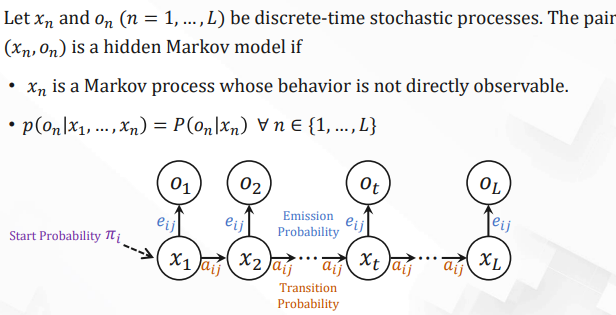
Hidden Markov Models (HMMs)
Understanding Bayes’ Rule:
- Prior $P(H)$ : How probable was our hypothesis before observing the evidence?
- Likelihood $p(E|H)$ : How probable is the evidence given that our hypothesis is true?
- Marginal $P(E)$: How probable is the new evidence?
| Notation | Explanation |
|---|---|
| $Q = \{q_1, \ldots, q_n\}$ | The set of $n$ hidden states. |
| $V = \{v_1, \ldots, v_v\}$ | The set of all possible observed values. |
| $A = [a_{ij}]_{n \times n}$ | Transition matrix. $a_{ij}$ is the probability of transitioning from state $i$ to state $j$. $\sum_{j=1}^n a_{ij} = 1 \, \forall i$. |
| $O = o_1 o_2 \cdots o_L$ | Observed sequence. $o_t \in V$. |
| $x = x_1 x_2 \cdots x_L$ | Hidden state sequence. $x_t \in Q$. |
| $E = [e_{ij}]_{n \times v}$ | Emission probability matrix. $e_{ij} = P(o = v_j \mid x = q_i)$ is the probability of observing $v_j$ at state $q_i$. $\sum_{j=1}^V e_{ij} = 1 \, \forall i$. |
| $\pi = [\pi_1, \pi_2, \ldots, \pi_n]$ | Start probability distribution. $\pi_i$ is the probability of Markov chain starting from $i$. $\sum_{i=1}^n \pi_i = 1$. |
Question #1 – Evaluation
The evaluation problem in HMM: Given a model $M$ and an observed sequence $O$, calculate the probability of the observed sequence $P(O|M)$ .
Forward Algorithm
Denote $\alpha_t(j)$ as the probability of observing $o_1 o_2 \ldots o_t$ and the hidden state at $t$ being $q_j$:
Obviously, $\alpha_t(j)$ can be rewritten as:
Define Initial Values:
Iterative solving:
Obtaining results:
Backward Algorithm
Denote $\beta_t(j)$ as the probability of observing $o_{t+1} o_{t+2} \ldots o_L$ and the hidden state at $t$ being $q_j$:
Obviously, $\beta_t(j)$ can be rewritten as:
Define Initial Values:
Iterative solving:
Obtaining results:
Question #2 – Decoding
The decoding problem in HMM: Given a model $M$ and an observed sequence $O$, calculate the most probable hidden state sequence $\mathbf{x} = \arg\max_{\mathbf{x}} p(\mathbf{x}, O | M)$.
Define:
According to the recurrence relation, rewrite the above as:
Therefore, the most probable hidden state sequence is:
Viterbi Algorithm
Define Initial Values:
Iterative solving:
Obtaining results:
Computational Complexity: $O(n^2 L)$
Question #3 – Learning
The learning problem in HMM: Given an observed sequence $O$, estimate the parameters of model: $M = \arg \max \limits_{M}P(M|O)$
For simplicity, in the following steps we only present the learning process of transition matrix $A$. (The other parameters can be learned in a similar manner.)
Baum-Welch Algorithm (a special case of EM algorithm)
- Expectation Step (E-step): Using the observed available data of the dataset, we estimate (guess) the values of the missing data with the current parameters $\theta_{\text{old}}$.
- Maximization Step (M-step): Using complete data generated after the E-step, we update the parameters of the model.
E-step
(#$T_{ij}$ denotes the times of hidden state transitioning from $q_i$ to $q_j$)
Generate the guesses of #$T_{ij}$, i.e., the expected counts:
Can be estimated with Forward Algorithm and Backward Algorithm.
M-step
Generate new estimations with the expected counts:
Estimation when hidden state is unknown.
Iterative Solving: Recalculate the expected counts with newly estimated parameters (E-step). Then generate newer estimations of $\theta$ with (M-step). Repeat until convergence.
Bayesian Networks
Naive Bayes
Naïve Bayes Assumption: Features $X_i$ are independent given class $Y$:
Inference: the label can be easily predicted with Bayes’ rule
$Y^*$ is the value that maximizes Likelihood $\times$ Prior.
When the number of samples is small, it is likely to encounter cases where $\text{Count}(Y = y) = 0$ or $\text{Count}(X_i = x, Y = y) = 0$. So we use Laplace Smoothing. The parameters of Naïve Bayes can be learned by counting:
- Prior:
- Observation Distribution
Here, $C$ is the number of classes, $S$ is the number of possible values that $X_i$ can take.
Learning & Decision on BN
Bayesian Network
BN$(G, \Theta)$: a Bayesian network
- $G$ is a DAG with nodes and directed edges.
- Each node represents a random variable. Each edge represents a causal relationship/dependency.
- $\Theta$ is the network parameters that constitute conditional probabilities.
- For a node $t$, its parameters are represented as $p(x_t \mid x_{\text{pa}(t)})$.
Joint probability of BN:
where $\text{pa}(t)$ is the set of all parent nodes of node $t$.
Learning on Bayesian Network
Notation: Suppose BN has $n$ nodes, we use $\text{pa}(t)$ to denote the parent nodes of $t$ $(t = 1, \ldots, n)$
By the conditional independence of BN, we have
Thus, the posterior becomes:
Learning BN with Categorical Distribution
Consider a case where each probability distribution in BN is categorical, In this case, we can model the conditional distribution of node $t$ as(We use a scalar value $c$ to represent parent nodes’ states for simplicity.):
and the conditional probability of node $t$ can be denoted as:
Categorical Distribution:
E.g., toss a coin $(d = 2)$, roll a die $(d = 6)$
Count the training samples where $x_t = k, x_{\text{pa}(t)} = c$:
According to the property of categorical distribution, we can represent the likelihood function as:
Thus the posterior can be further factorized:
Notation:
- $D_{tc}$ are the sample set where the value of $x_{\text{pa}(t)}$ is $c$
- $q_t$ is the number of possible values of $x_{\text{pa}(t)}$
- $K_t$ is the number of possible values of $x_t$
How to choose the probability distribution function for the prior $p(\theta_{tc})$? It would be highly convenient if the posterior shares the same form as the prior.
Conjugate Prior: A prior distribution is called a conjugate prior for a likelihood function if the posterior distribution is in the same probability distribution family as the prior.
The conjugate prior for the categorical distribution is the Dirichlet distribution:
Choosing the prior as conjugate prior — Dirichlet distribution:
$\alpha_{tck}$ are integers and are the hyperparameters of BN model.
In this case, the posterior can be easily derived as:
We can then derive an estimate of $\theta_{tck}$ by calculating the expectation:
K-Means Algorithm
- Initalize cluster centers $\mu_1, \cdots, \mu_k$ randomly.
Repeat until no change of cluster assignment
- Assignment step: Assign data points to closest cluster center
- Update Step: Change the cluster center to the average of its assigned points
Optimization View of K-Means
Optimization Objective: within-cluster sum of squares (WCSS)
Step 1: Fix $\mu$, optimize $r$
Step 2: Fix $r$, optimize $\mu$
Rule of Thumbs for initializing k-means
- Random Initialization: Randomly generate 𝑘 points in the space.
- Random Partition Initialization: Randomly group the data into 𝑘 clusters and
use their cluster center to initialize the algorithm. - Forgy Initialization: Randomly select 𝑘 samples from the data.
- K-Means++: Iteratively choosing new centroids that are farthest from the existing
centroids.
How to tell the right number of clusters?
We find the elbow point of the $J_e$ image.
EM Algorithm for Gaussian Mixture Model (GMM)
Multivariate Gaussian Distribution
$d$-dimensional Multivariate Gaussian:
- $\mu \in \mathbb{R}^d$ the mean vector
- $\Sigma \in \mathbb{R}^{d \times d}$ the covariance matrix
MLE of Gaussian Distribution
The likelihood function of a given dataset $X = \{x_1, x_2, \ldots, x_N\}$:
The maximum likelihood estimation (MLE) of the parameters is defined by:
The optimization problem of maximum likelihood estimation (MLE):
Solve the optimization by taking the gradient:
Gaussian Mixture Model (GMM)
A Gaussian Mixture Model (GMM) is the weighted sum of a family of Gaussians whose density function has the form:
- Each Gaussian $N(\mu_k, \Sigma_k)$ is called a component of GMM.
- Scalars $\{\pi_k\}_{k=1}^{K}$ are referred to as mixing coefficients, which satisfy
This condition ensures $p(x \mid \pi, \mu, \Sigma)$ is indeed a density function.
Soft Clustering with Mixture Model
By Bayes Rule, the posterior probability of $z$ given $x$ is:
We call $\gamma_k$ the responsibility of the $k$-th component on the data $x$.
Probabilistic Clustering: each data point is assigned a probability distribution over the clusters.
“$x$ belongs to the $k$-th cluster with probability $\gamma_k$”
MLE for Gaussian Mixture Model
Log-likelihood function of GMM
Maximum Likelihood Estimation
subject to:
Optimality Condition for $\mu$
Take partial derivative with respect to $\mu_k$,
Notice that the posterior of $z_n$ (also known as responsibility $\gamma_{n,k}$) can be written as
Thus
Optimality Condition for $\Sigma$
Similarly, take derivative with respect to $\Sigma_k$, which yields
Responsibility-reweighted Sample Covariance
Optimality Condition for $\pi$
Constraints of mixing coefficients $\pi$: $\sum_{k=1}^{K} \pi_k = 1$
Introduce Lagrange multiplier:
Take derivative with respect to $\pi_k$, which gives
By the constraints, we have $1 = \sum_{k=1}^{K} \pi_k = \frac{-1}{\lambda} \sum_{k=1}^{K} N_k$,
Also notice that
Therefore,
Expectation-Maximization (EM) Algorithm
- Initialize $\pi_k, \mu_k, \Sigma_k, \quad k = 1, 2, \ldots, K$
- E-Step: Evaluate the responsibilities using the current parameter values
- M-Step: Re-estimate the parameters using the current responsibilities
where $N_k = \sum_{n=1}^{N} \gamma_{n,k}$
- Return to step 2 if the convergence criterion is not satisfied.
Hierarchical Clustering
Distance Function: The distance function affects which pairs of clusters are merged/split and in what order.
- Single Linkage:
- Complete Linkage:
- Average Linkage:
Two Types of Hierarchical Clustering
Bottom-Up (Agglomerative)
- Start with each item in its own cluster, find the best pair to merge into a new cluster.
- Repeat until all clusters are fused together.
Top-Down (Divisive)
- Start with one all-inclusive cluster, consider every possible way to divide the cluster in two.
- Choose the best division and recursively operate on both sides.
Agglomerative (Bottom-up) Clustering
- Input: cluster distance measure $d$, dataset $X = \{x_n\}_{n=1}^{N}$, number of clusters $k$
- Initialize $\mathcal{C} = \{C_i = \{x_n\} \mid x_n \in X\}$ // Each point in separate cluster
- Repeat:
- Find the closest pair of clusters $C_i, C_j \in \mathcal{C}$ based on distance metric $d$
- $C_{ij} = C_i \cup C_j$ // Merge the selected clusters
- $\mathcal{C} = (\mathcal{C} \setminus \{C_i, C_j\}) \cup \{C_{ij}\}$ // Update the clustering
- Until $|\mathcal{C}| = k$
A naïve implementation takes space complexity $O(N^2)$, time complexity $O(N^3)$.
LASSO Regression
LASSO (Least Absolute Shrinkage and Selection Operator): Simply linear regression with an $\ell_1$ penalty for sparsity
sparse solution $\leftrightarrow$ feature selection
Principal Component Analysis (PCA)
Computing PCA: Eigenvalue Decomposition
Objective: Maximize variance of projected data
subject to $\mathbf{u}_j^T \mathbf{u}_j = 1$, $\mathbf{u}_j^T \mathbf{u}_k = 1$, $k < j$
Observation: PC $j$ is direction of the $j$-th largest eigenvector of $\frac{1}{n} \mathbf{X}^T \mathbf{X}$
Eigenvalue Decomposition:
are eigenvectors of $\frac{1}{n} \mathbf{X}^T \mathbf{X}$
Manifold Learning
Geodesic distance: lines of shortest length between points on a manifold